Where’s my data?

If you go to your AWS s3 bucket you’ll see a few files there, but nothing that looks like your household data.

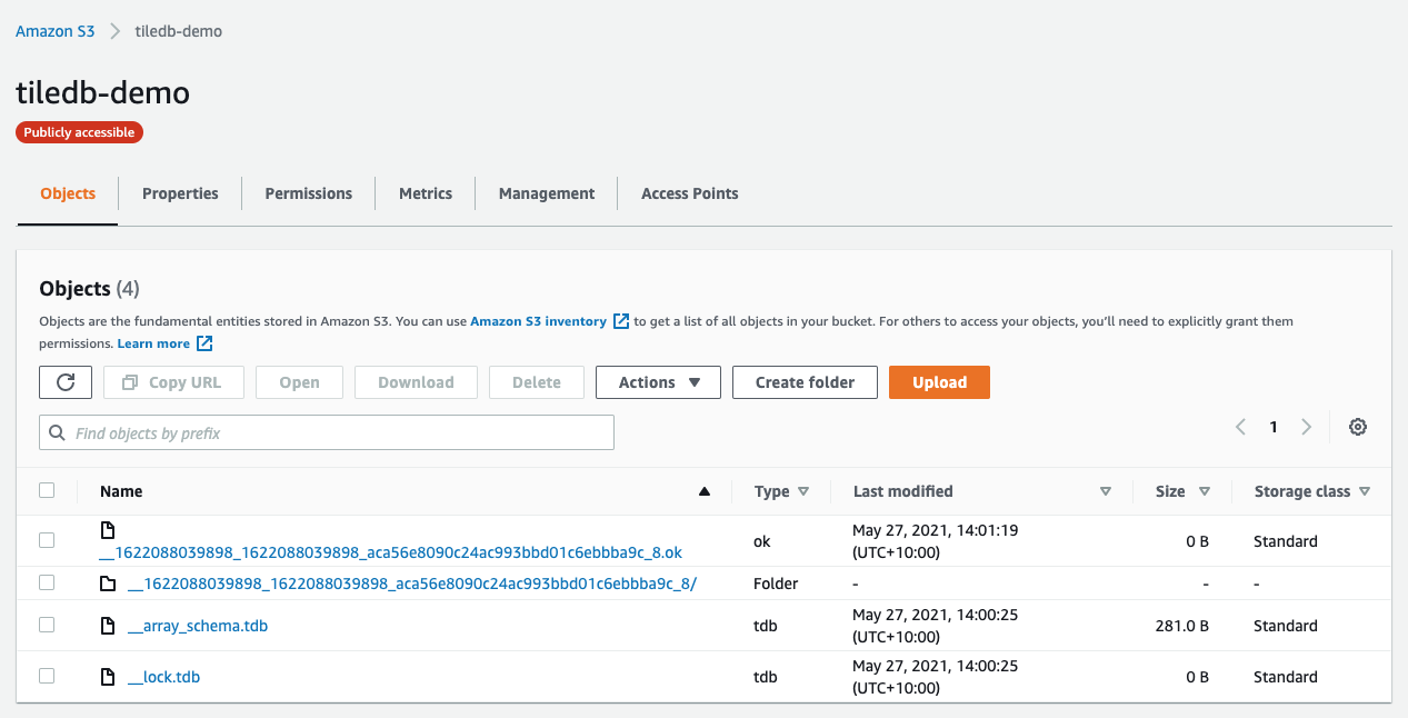
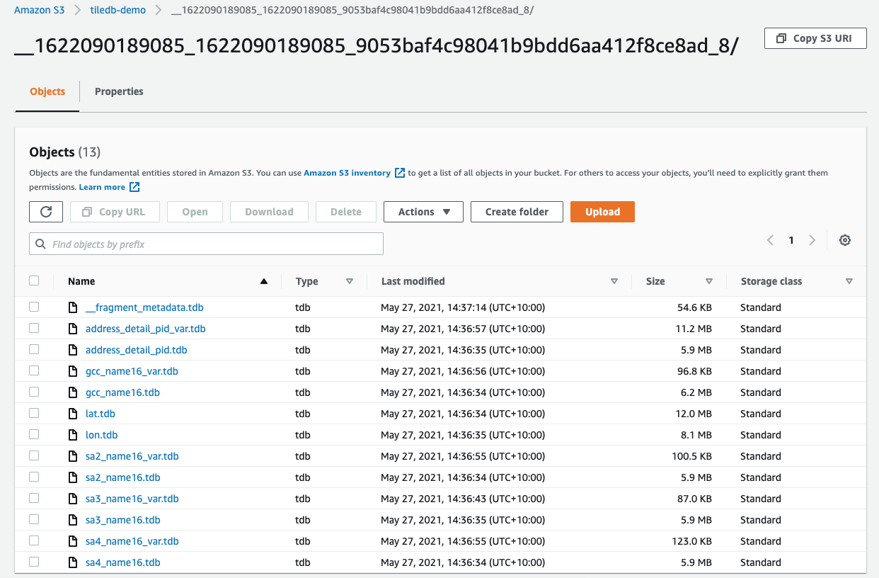
Someone a lot smarter than me can tell you exactly what all the files are for, but from a layman’s perspective (i.e., mine), all I need to know is TileDB has done the hard work of converting my data into a format it understands.

And indeed we can see each column in the data has it’s own .tdb file

Querying TileDB

The first thing you need to do is create an Array object.

arr <- tiledb::tiledb_array(uri_s3, as.data.frame = TRUE)

This doesn’t actually hold any data, but it does point to the data

arr

tiledb_array
  uri                = 's3://tiledb-demo/'
  is.sparse          = TRUE
  as.data.frame      = TRUE
  attrs              = (none)
  selected_ranges    = (none)
  extended           = TRUE
  query_layout       = (none)
  datetimes_as_int64 = FALSE
  encryption_key     = (none)
  timestamp          = (none)
  as.matrix          = FALSE

You can get all the data back out of the Array by ‘subsetting it’

df <- arr[]

head( df )

  sa4_name16 sa3_name16 sa2_name16      lon       lat   gcc_name16
1   Ballarat   Ballarat  Alfredton 143.6962 -37.53143 Rest of Vic.
2   Ballarat   Ballarat  Alfredton 143.6964 -37.55797 Rest of Vic.
3   Ballarat   Ballarat  Alfredton 143.6964 -37.55797 Rest of Vic.
4   Ballarat   Ballarat  Alfredton 143.6964 -37.55797 Rest of Vic.
5   Ballarat   Ballarat  Alfredton 143.6982 -37.55781 Rest of Vic.
6   Ballarat   Ballarat  Alfredton 143.6982 -37.55781 Rest of Vic.

nrow( df )
[1] 5502355

This has returned all the data to R. If you want to query only subsets of the data you need to define the ‘ranges’ you want returned.

If you come from a SQL background you would normally write a query like

SELECT * 
  FROM tbl_household
    WHERE lon >= 143.0 
    AND lon <= 144.0
    AND lat >= -38.9
    AND lat <= -38.2
    ;

In the TileDB-world you specify the ranges on the array

tiledb::selected_ranges(arr) <- list(
  lon = cbind(143.96, 144.1)
  , lat = cbind(-38.9, -38.2)
  )

arr@selected_ranges

$lon
       [,1]  [,2]
[1,] 143.96 144.1

$lat
      [,1]  [,2]
[1,] -38.9 -38.2

And now calling the ‘subset’ method will return just those defined ranges

df <- arr[]

head( df )

  sa4_name16    sa3_name16 sa2_name16      lon       lat   gcc_name16
1    Geelong Barwon - West Winchelsea 143.9607 -38.37917 Rest of Vic.
2    Geelong Barwon - West Winchelsea 143.9611 -38.23718 Rest of Vic.
3    Geelong Barwon - West Winchelsea 143.9611 -38.23718 Rest of Vic.
4    Geelong Barwon - West Winchelsea 143.9611 -38.24019 Rest of Vic.
5    Geelong Barwon - West Winchelsea 143.9611 -38.24019 Rest of Vic.
6    Geelong Barwon - West Winchelsea 143.9611 -38.24019 Rest of Vic.

nrow( df )
[1] 4232

Which matches our original data

dt_households[
  lon >= 143.96 & lon <= 144.1 & 
    lat >= -38.9 & lat <= -38.2 
][
  , .N  ## in data.table, .N == base::nrow() == dplyr::n()
]

[1] 4232

And here’s an example using a character column in the query. However, a quirk with constructing this query is you need to use the same values twice.

m <- matrix(
  data = c(
    rep("Melbourne - Inner", 2)
    , rep("Melbourne - South East", 2)
  )
  , ncol = 2
  , byrow = T
)

tiledb::selected_ranges(arr) <- list(
  sa4_name16 = m
  )

df <- arr[]

head( df )
         sa4_name16         sa3_name16 sa2_name16      lon       lat        gcc_name16
1 Melbourne - Inner Brunswick - Coburg  Brunswick 144.9488 -37.76973 Greater Melbourne
2 Melbourne - Inner Brunswick - Coburg  Brunswick 144.9488 -37.76973 Greater Melbourne
3 Melbourne - Inner Brunswick - Coburg  Brunswick 144.9489 -37.76987 Greater Melbourne
4 Melbourne - Inner Brunswick - Coburg  Brunswick 144.9489 -37.76987 Greater Melbourne
5 Melbourne - Inner Brunswick - Coburg  Brunswick 144.9491 -37.77546 Greater Melbourne
6 Melbourne - Inner Brunswick - Coburg  Brunswick 144.9491 -37.77542 Greater Melbourne

unique( df$sa4_name16 )
[1] "Melbourne - Inner"      "Melbourne - South East"

nrow( df )
[1] 1247517

dt_households[
  sa4_name16 %in% unique( as.vector( m ) )
][
  , .N
]

[1] 1247517