A case study in using deep learning to identify fraud
How can deep learning help to identify fraud?
Identifying unusual or suspicious observations can be challenging, particularly when such events are very rare. In this case study we’ll explain how we used deep learning to identify unusual transactions for a client. Because we can’t show you their data, for this example we’ll the Kaggle Credit Card Fraud dataset.
Only 0.17% of transactions in the dataset are known fraud. With this sort of imbalance, it’s very difficult to reliably train a supervised model to recognise ‘fraud’. Instead, we’ll use an autoencoder (a type of artificial neural network) to identify unusual transactions.
Importantly, we don’t want to just identify suspicious transactions, but also associate those transactions with customers. While a single suspicious transaction may not be cause for concern, a pattern of unusual transactions could suggest fraud. Linking suspicious transactions to a card holder provides more context for deciding whether to pursue these transactions further.
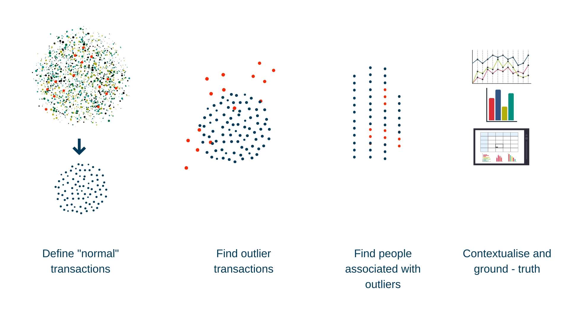
In this case study we will use deep learning to define normal transactions, use this model to identify suspicious transactions, and associate those transactions with individual cards. This places the questionable transactions in context to improve decision making.
How do autoencoders work?
An autoencoder learns to represent its inputs using a small number of dimensions and to reconstruct them from this compressed form. Ideally this reconstruction will be very similar to the original input, indicating that the autoencoder is able to capture the most important elements of the input while reducing the amount of noise. The difference between reconstruction and output in each iteration (known as reconstruction error) is used to help the model refine its representation. This is a type of unsupervised learning, as the model is trained without class labels.
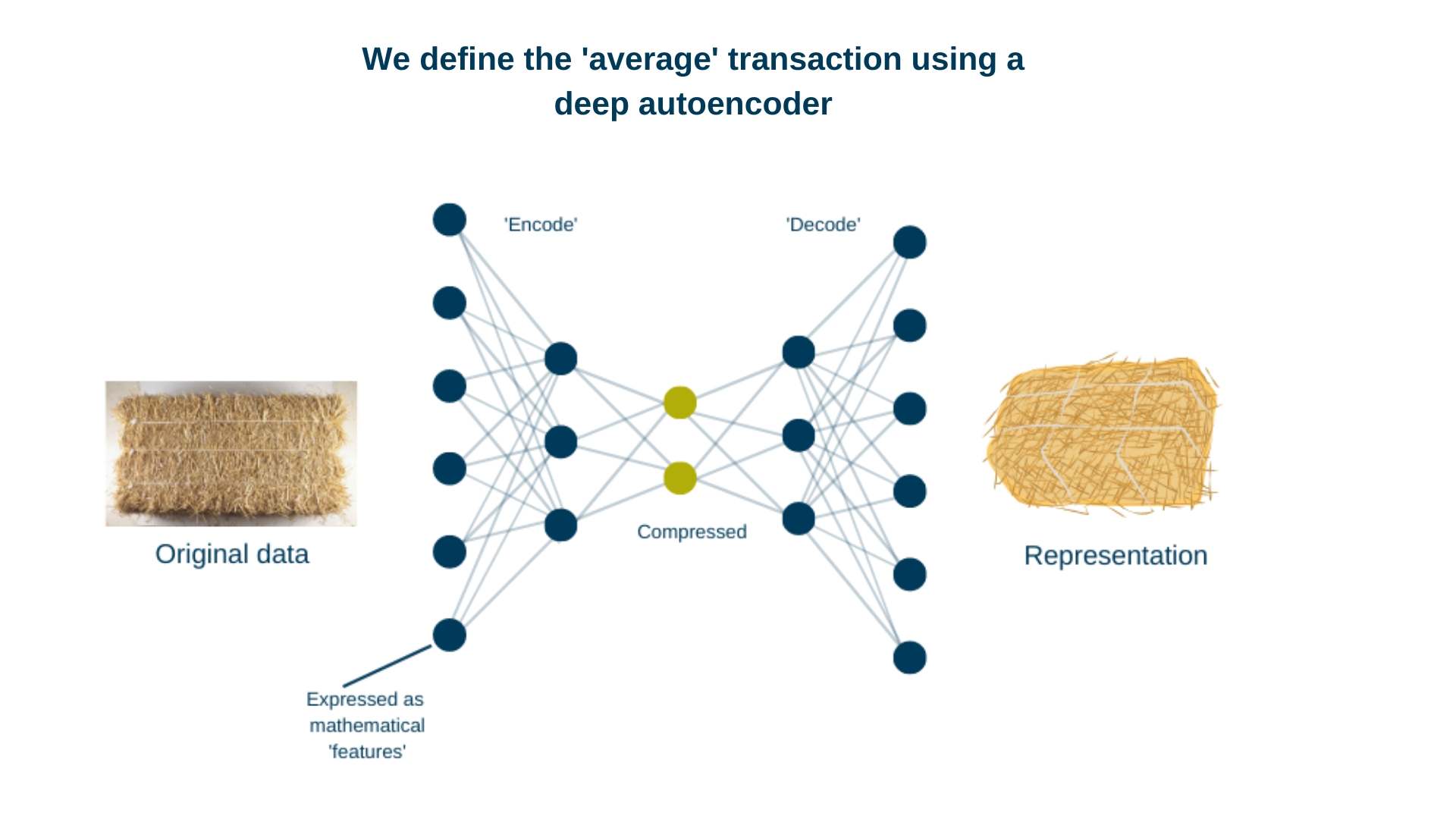
Because the vast majority of transactions are non-fraudulent, the model can represent and reconstruct these transactions well. We expect fraudulent and non-fraudulent transactions will have subtly different characteristics, such as combinations of values that only occur in one or the other. Because there are so few fraudulent transactions in the data, the autoencoder should be worse at representing them. This means we can use the reconstruction errors to identify potential fraud. These anomalous transactions should in general have higher reconstruction errors.
The data
The data we’re using is available from Kaggle. It contains 284,807 transactions (rows) of 33 features (columns), including (integer) time and decimal dollar transaction amount. The Class column is a boolean integer that indicates if the translation is a fraud or not. The remaining columns are (unspecified) transaction features.
| card_no | txn_id | Time | Amount | Class |
|---|---|---|---|---|
| 4568 | 1 | 0 | 149.62 | 0 |
| 3630 | 2 | 0 | 2.69 | 0 |
| 1762 | 3 | 1 | 378.66 | 0 |
| 1336 | 4 | 1 | 123.50 | 0 |
| 866 | 5 | 2 | 69.99 | 0 |
| 732 | 6 | 2 | 3.67 | 0 |
Although the original Kaggle data doesn’t have any card holder information, here we’ve associated each transaction with a synthetic card holder. We won’t include the card numbers in our model so we can treat each transaction as independent, but later on we can explore how many anomalous transactions are associated with each card.
Of the 284,807 transactions, only 492 are known fraud. Each transaction is associated with a single card number, with only 50 of the 5000 cards have any fraudulent transactions on them.
Importantly, even for cards with fraudulent transactions, there are also many non-fraudulent ones. The worst offender has 27% flagged as fraudulent.
Our approach
We trained our autoencoder to identify typical transactions using TensorFlow (via the keras R package). The architecture we’re using is based on one described in a preprint by Schreyer et al., where they use deep learning to help identify accounting fraud. A simpler example of training an autoencoder on the same dataset is described in this RStudio blog post.
Identifying suspicious transactions
Once we trained our model, we calculated reconstruction errors associated with each transaction. Remember: the basis of our approach to identify fraudulent transactions is that they will generally have relatively high reconstruction errors.
The next step is to select a threshold for the reconstruction error, which defines a suspicious transaction. For this we need to consider both precision and recall.
Precision is the proportion of all transactions that we label as suspicious (on the basis of the model’s prediction) that really are fraudulent. In contrast, recall is the proportion of all transactions that really are fraudulent that we correctly identify.
Ideally both precision and recall will be high, but there is often a trade off and which you care more about will depend on the specific problem. Since in this case we’re aiming to identify potential fraud, it’s more important to not miss any suspicious transactions than it is to avoid mis-identifying innocent transactions. So we care more about having high recall than high precision.
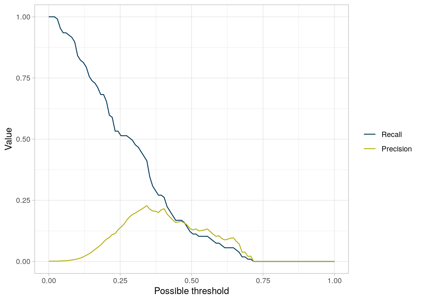
The plot shows how precision and recall change depending on what threshold we set. This can help us identify an appropriate one. In this case, precision is highest at a threshold of ~0.35, but the recall at this threshold is not very good (~0.3). Choosing a threshold of 0.2 gives us better recall at the cost of slightly worse precision.
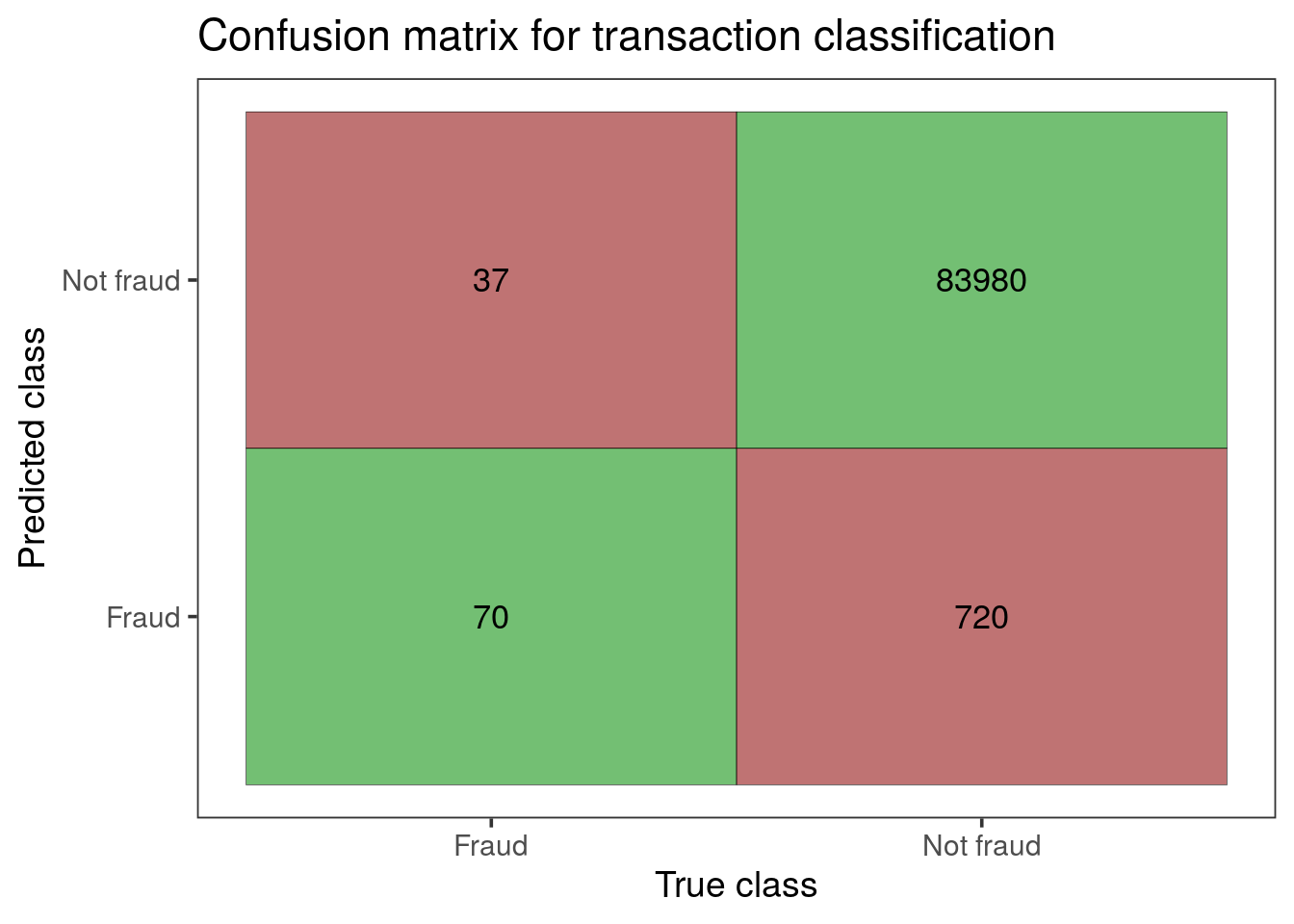
From the confusion matrix we can confirm that at this threshold we’re correctly classifying most fraudulent transactions. However, we’re also incorrectly classifying many non-fraudulent transactions.
Linking suspicious transactions to card holders
Up until this point we’ve treated each transaction as independent, but in fact each transaction is associated with a card number. Just as we identified transactions that were outliers, we can identify customers that are outliers in terms of their number of suspicious transactions. This means we can identify potential fraud at the customer level as well as at the transaction level.
If a high proportion of transactions associated with one card number are flagged as potentially fraudulent, we should feel more confident that a customer should be investigated than if they have only one potentially problematic transaction. However, it’s likely that even customers committing fraud also have many non-fraudulent transactions.
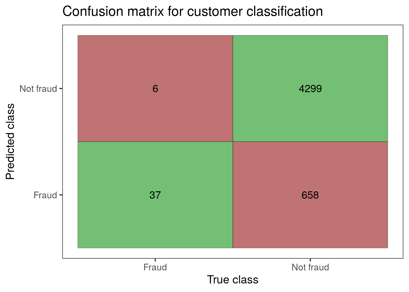
If we flag a card for having even one suspicious transaction, we correctly identify most of the cards that do really have a fraudulent transaction. We also incorrectly flag a lot of cards, though in this scenario it’s better than missing a large number of card holders who are really making fraudulent transactions.
Applying deep learning to solve real world problems
We’ve shown you a fairly straightforward example of using an autoencoder to identify unusual transactions, but the real life version of this problem was much trickier. We spent a lot of time auditing and processing our client’s data to make sure we could get the most out of this approach, whereas the data we used in this example needed little pre-processing. We also needed to refine many of the parameters of the model and test different architectures to find one that performed well.
As you can see, deep learning is a powerful approach for identifying anomalies. If you’d like to learn more about how we could help you apply techniques like this in your organisation, please get in touch .
