Visualising spatial data using sf and mapdeck - part one
I just started as intern at Symbolix and am completely new to spatial data, so I spent the first few days of my internship learning how to use some of the tools of the trade. I’m going to be writing up what I’ve learned as a series of blog posts focusing on visualising spatial data.
In this post I’ll give a very brief introduction to spatial data, and in my next post I’ll start working through an example using GPS data from migrating birds.
A very brief introduction to visualising spatial data in R
If you have spatial data, the first thing you’ll likely want to do is visualise it. In R there are a lot of different packages to choose from, including ggplot2, tmap, and leaflet.
However, here I’m going to focus on plotting in mapdeck, which allows you to make great-looking interactive maps and includes some plotting options that are not available in many of the other offerings.
See for yourself by zooming, tilting (Ctrl+drag) and panning around this arc-layer.
But before we get to plotting, we need to understand…
What is spatial data?
The package sf is widely used to work with spatial data in R. sf stands for ‘simple features’, which is a formal standard for representing spatial data. There are many geometry types, but the ones you’re most likely to come across are point, linestring, and polygon (and their counterparts multipoint, multilinestring, and multipolygon).
You’re probably already familiar with vectors, matrices, and lists. And you probably already know how to build heirarchies of objects using these structures
v1 <- c(1,2)
v2 <- c(2,2)
v3 <- c(2,3)
v4 <- c(1,3)

m <- matrix( c(v1, v2, v3, v4, v1), ncol = 2, byrow = T)

l <- list( m )

v1; v2; v3; v4; m; l## [1] 1 2## [1] 2 2## [1] 2 3## [1] 1 3## [,1] [,2]
## [1,] 1 2
## [2,] 2 2
## [3,] 2 3
## [4,] 1 3
## [5,] 1 2## [[1]]
##      [,1] [,2]
## [1,]    1    2
## [2,]    2    2
## [3,]    2    3
## [4,]    1    3
## [5,] 1 2And I’m sure you already know about data.frames
df <- data.frame(
    val = c( "a", "b" )
    , x = c( v1[1], v2[1] )
    , y = c( v1[2], v2[2] )
)
df## val x y
## 1 a 1 2
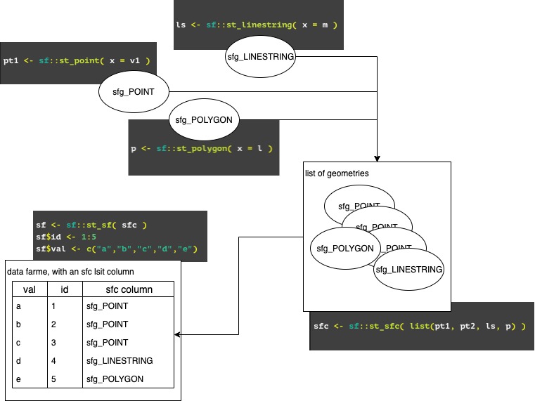
## 2 b 2 2Well, an sf object is simply some combination of these (with some attributes attached, but that’s for another time). Specifically, an sf object is built from
- sfg - a single geometry
- point is a vector
- linestring is a matrix
- polygon is a list of matrices
- sfc - a list of sfgs
- sf - data.frame with at least one geometry column (the sfc object)
So with our objects we’ve just built, v1 to v4 are points, m is a linestring, and l is a polygon.
library(sf)pt1 <- sf::st_point( x = v1 )
pt2 <- sf::st_point( x = v2 )
pt3 <- sf::st_point( x = v3 )
pt4 <- sf::st_point( x = v4 )
ls <- sf::st_linestring( x = m )
p <- sf::st_polygon( x = l )
pt1; pt2; ls; p## POINT (1 2)## POINT (2 2)## LINESTRING (1 2, 2 2, 2 3, 1 3, 1 2)## POLYGON ((1 2, 2 2, 2 3, 1 3, 1 2))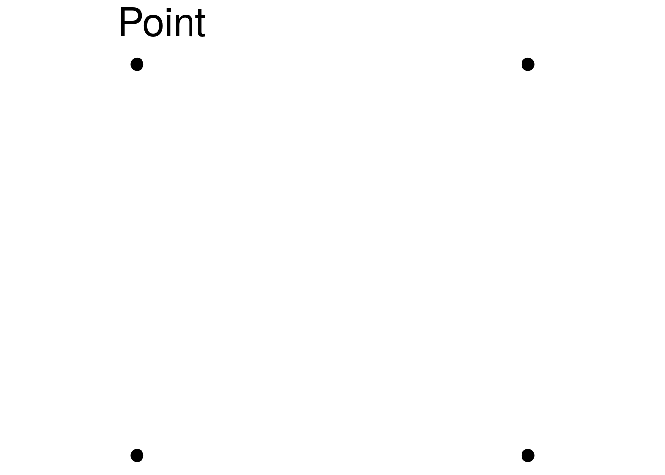
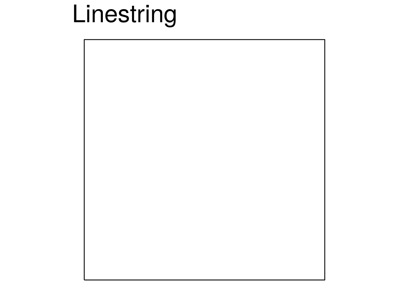
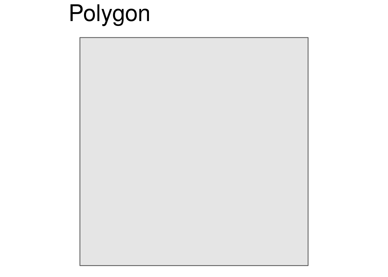
See these are simply our vectors, matrix and list (with some extra attributes attached). We can get back to the original structure by removing the sfg class
unclass(pt1)## [1] 1 2unclass(ls)## [,1] [,2]
## [1,] 1 2
## [2,] 2 2
## [3,] 2 3
## [4,] 1 3
## [5,] 1 2unclass(p)## [[1]]
##      [,1] [,2]
## [1,]    1    2
## [2,]    2    2
## [3,]    2    3
## [4,]    1    3
## [5,] 1 2Given an sfc is a collection of sfg objects, we can combine these into a list and make one
sfc <- sf::st_sfc( list(pt1, pt2, ls, p) )


sfc## Geometry set for 4 features
## geometry type: GEOMETRY
## dimension: XY
## bbox: xmin: 1 ymin: 2 xmax: 2 ymax: 3
## CRS: NA## POINT (1 2)## POINT (2 2)## LINESTRING (1 2, 2 2, 2 3, 1 3, 1 2)## POLYGON ((1 2, 2 2, 2 3, 1 3, 1 2))And again we can remove the sfc class to get back our vectors, matrix and list
lapply( sfc, unclass )## [[1]]
## [1] 1 2
##
## [[2]]
## [1] 2 2
##
## [[3]]
## [,1] [,2]
## [1,] 1 2
## [2,] 2 2
## [3,] 2 3
## [4,] 1 3
## [5,] 1 2
##
## [[4]]
## [[4]][[1]]
## [,1] [,2]
## [1,] 1 2
## [2,] 2 2
## [3,] 2 3
## [4,] 1 3
## [5,] 1 2And finally, an sf object is a data.frame with an sfc object as one of the columns
sf <- sf::st_sf( sfc )
sf## Simple feature collection with 4 features and 0 fields
## geometry type: GEOMETRY
## dimension: XY
## bbox: xmin: 1 ymin: 2 xmax: 2 ymax: 3
## CRS: NA
## sfc
## 1 POINT (1 2)
## 2 POINT (2 2)
## 3 LINESTRING (1 2, 2 2, 2 3, ...
## 4 POLYGON ((1 2, 2 2, 2 3, 1 ...Usually when working with spatial data, you’ll be interested not just in the geometries, but also the attributes of these geometries. These attributes can be stored in the sf dataframe and can be manipulated basically like any other dataframe.
sf$my_value <- c("a","b","c","d")
sf## Simple feature collection with 4 features and 1 field
## geometry type: GEOMETRY
## dimension: XY
## bbox: xmin: 1 ymin: 2 xmax: 2 ymax: 3
## CRS: NA
## sfc my_value
## 1 POINT (1 2) a
## 2 POINT (2 2) b
## 3 LINESTRING (1 2, 2 2, 2 3, ... c
## 4 POLYGON ((1 2, 2 2, 2 3, 1 ... d## subset just like a data.frame
sf[ sf$my_value %in% c("a","c"), ]## Simple feature collection with 2 features and 1 field
## geometry type: GEOMETRY
## dimension: XY
## bbox: xmin: 1 ymin: 2 xmax: 2 ymax: 3
## CRS: NA
## sfc my_value
## 1 POINT (1 2) a
## 3 LINESTRING (1 2, 2 2, 2 3, ... clibrary(dplyr)## or use in a dplyr chain
sf %>% filter( my_value %in% c("b","d") )## Simple feature collection with 2 features and 1 field
## geometry type: GEOMETRY
## dimension: XY
## bbox: xmin: 1 ymin: 2 xmax: 2 ymax: 3
## CRS: NA
## sfc my_value
## 1 POINT (2 2) b
## 2 POLYGON ((1 2, 2 2, 2 3, 1 ... dHere’s a graphic showing the basic structure of how these objects are built up.
In my next few posts I’ll give a few examples on how to plot spatial data using mapdeck.
Useful resources
- https://cran.r-project.org/web/packages/sf/
The documentation for sf, which includes several very helpful vignettes that highlight the range of things you can do using sf. - https://symbolixau.github.io/mapdeck/articles/mapdeck.html
The documentation for mapdeck, which includes a lot of examples. The “Why isn’t it working?” page will likely address whatever problems you run into. - https://geocompr.robinlovelace.net/
“Geocomputation with R” goes into great depth and covers many different tools. Very useful to consult if you’re confused by something like coordinate reference systems. - https://www.jessesadler.com/post/simple-feature-objects/
This is a great blog post about sf and how you can use it to look at spatial data. Other posts on this blog are also very relevant. - https://cengel.github.io/R-spatial/
Materials from a workshop on spatial data in R that include very practical advice on the main things you can do with spatial data.
